🌐 中文 English
This article aims to provide an explanation of the algorithm implementation for the Fibonacci sequence.
Do You Really Understand the Fibonacci Sequence Algorithm?
Test link for this chapter: https://leetcode.cn/problems/fibonacci-number/
What is the Fibonacci Sequence?
The Fibonacci sequence, also known as the golden ratio sequence, is a sequence introduced by the Italian mathematician Leonardo Fibonacci using the example of rabbit reproduction. Its values are: 1, 1, 2, 3, 5, 8, 13, 21, 34... Mathematically, this sequence is defined by the following recurrence relation:
F(0)=0, F(1)=1, F(n)=F(n-1)+F(n-2) (n ≥ 2, n ∈ N*).
Algorithm Implementation of the Fibonacci Sequence
Recursive Implementation
This is the most intuitive implementation method. Most people think of this approach first, as it is the simplest and easiest to write:
1
2
3
4
5
6
7
8
9
10
11
12
13
14
class Solution {
public:
    int fib(int n) {
        if (n == 0)
        {
            return 0;
        }
        if (n == 1)
        {
            return 1;
        }
        return fib(n - 1) + fib(n - 2);
    }
};
Test results (from LeetCode):
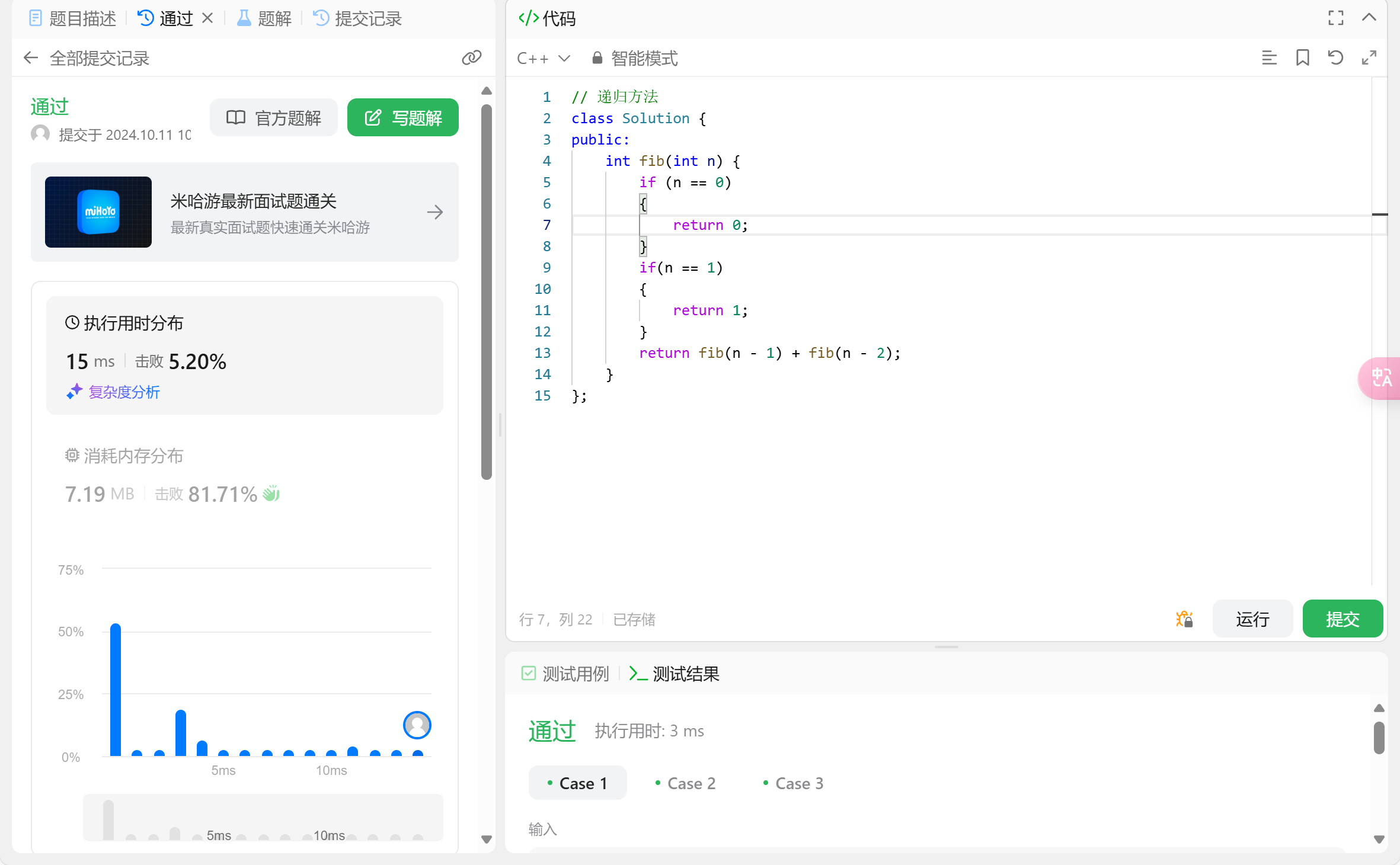 Because its time complexity is
 O(2^n), it appears very slow in the image, so I do not recommend using it.
Dynamic Programming Implementation
This is an implementation that trades space for time, with a time complexity of O(n). It can be divided into three implementation methods:
- Bottom-Up
- Top-Down
- Space-Optimized (Top-Down)
1. Bottom-Up
1
2
3
4
5
6
7
8
9
10
11
12
13
14
15
16
17
18
19
20
21
22
23
24
25
26
class Solution {
public:
    vector<int> dp;  // Reverse DP processing
    int f(int i)
    {
        if (i == 0)
        {
            return 0;
        }
        if (i == 1)
        {
            return 1;
        }
        if (dp[i] != -1)
        {
            return dp[i];
        }
        int ans = f(i - 1) + f(i - 2);
        dp[i] = ans;
        return ans;
    }
    int fib(int n) {
        dp = vector<int>(n + 1, -1);
        return f(n);
    }
};
2. Top-Down
1
2
3
4
5
6
7
8
9
10
11
12
13
14
15
16
17
18
19
20
21
class Solution {
public:
    vector<int> dp;
    int fib(int n) {
        if (n == 0)
        {
            return 0;
        }
        if (n == 1)
        {
            return 1;
        }
        dp = vector<int>(n + 1, 0);
        dp[1] = 1;
        for (int i = 2; i <= n; ++i)  // Using a for loop for forward processing
        {
            dp[i] = dp[i - 1] + dp[i - 2];
        }
        return dp[n];
    }
};
3. Space-Optimized (Top-Down)
1
2
3
4
5
6
7
8
9
10
11
12
13
14
15
16
17
18
19
20
21
22
23
class Solution {
public:
    int lastLast, last;    // Using two variables instead of dp to optimize space
    int fib(int n) {
        if (n == 0)
        {
            return 0;
        }
        if (n == 1)
        {
            return 1;
        }
        lastLast = 0;
        last = 1;
        for (int i = 2, tmp; i <= n; ++i)
        {
            tmp = last;
            last = last + lastLast;
            lastLast = tmp;
        }
        return last;
    }
};
These three methods:
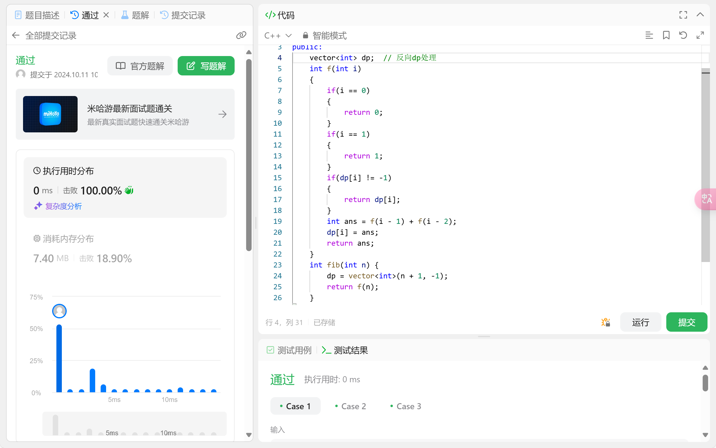
The first uses recursion + reverse DP
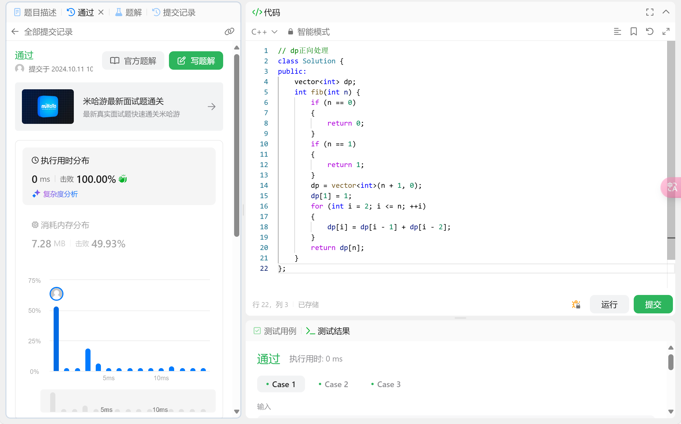
The second uses forward DP
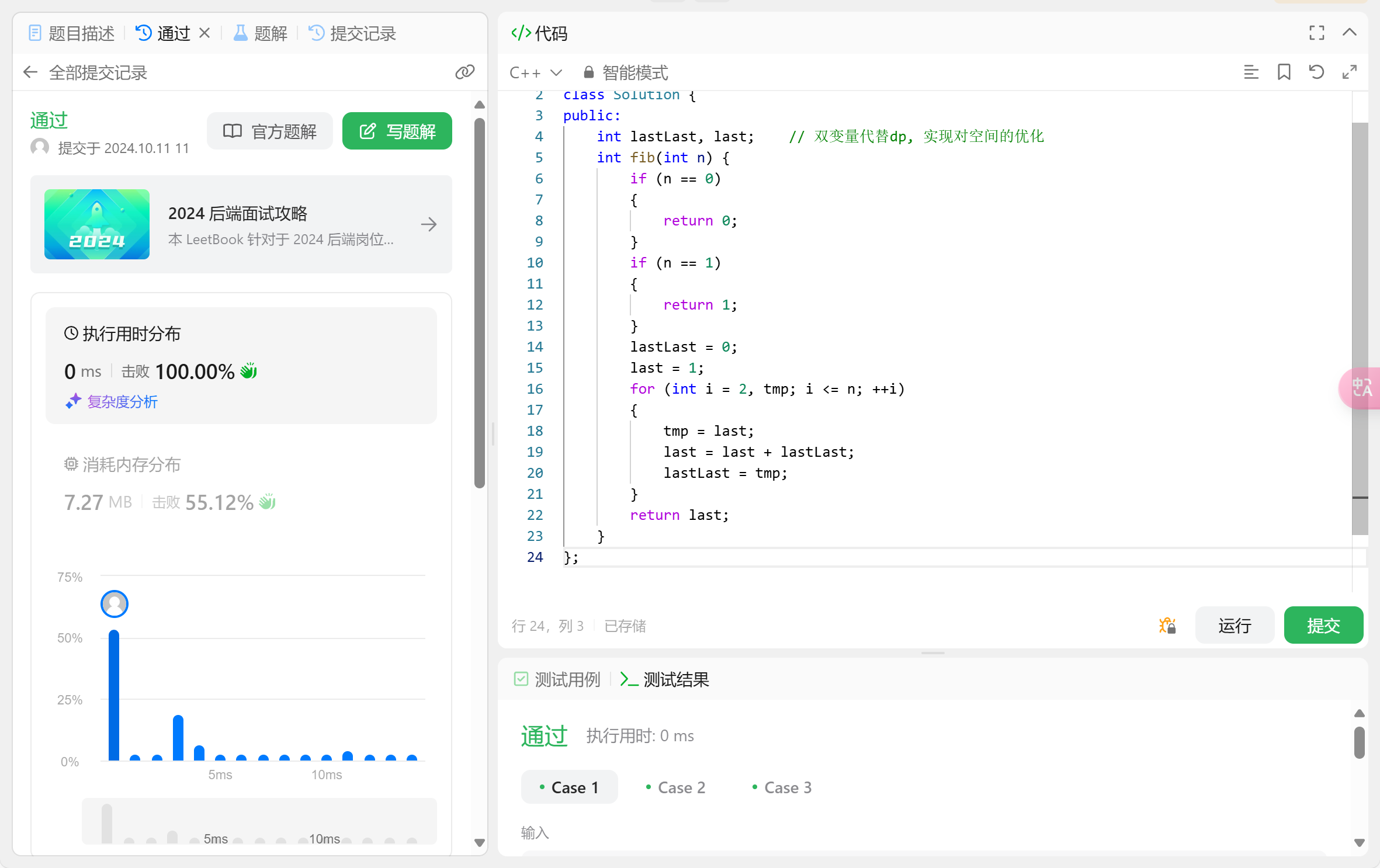
The third uses two variables instead of DP to optimize space
However, regardless of which method, their time complexity is O(n). In data testing, 0ms is no problem at all, and the implementation code is not difficult. These are the most commonly used implementation methods by most algorithm competition participants.
Matrix Fast Exponentiation Implementation
This is probably the most challenging part of this chapter. Its time complexity is O(logn), making it one of the fastest algorithms for implementing the Fibonacci sequence. The implementation is as follows:
1
2
3
4
5
6
7
8
9
10
11
12
13
14
15
16
17
18
19
20
21
22
23
24
25
26
27
28
29
30
31
32
33
34
class Solution {
public:
    // Matrix multiplication
    vector<vector<long long>> mult(vector<vector<long long>>& a, vector<vector<long long>>& b) {
        vector<vector<long long>> res(2, vector<long long>(2, 0));
        // Operation rules for two 2D matrices
        res[0][0] = a[0][0] * b[0][0] + a[0][1] * b[1][0];
        res[0][1] = a[0][0] * b[0][1] + a[0][1] * b[1][1];
        res[1][0] = a[1][0] * b[0][0] + a[1][1] * b[1][0];
        res[1][1] = a[1][0] * b[0][1] + a[1][1] * b[1][1];
        return res;
    }

    // Matrix fast exponentiation
    vector<vector<long long>> matrixPow(vector<vector<long long>> a, int n) {
        vector<vector<long long>> result = { {1, 0}, {0, 1} }; // Identity matrix
        while (n > 0) {
            if (n & 1) {
                result = mult(result, a);
            }
            a = mult(a, a);
            n >>= 1;
        }
        return result;
    }

    // Calculate the nth Fibonacci number
    int fib(int n) {
        if (n == 0) return 0;
        vector<vector<long long>> base = { {1, 1}, {1, 0} };
        vector<vector<long long>> result = matrixPow(base, n - 1);
        return result[0][0];
    }
};
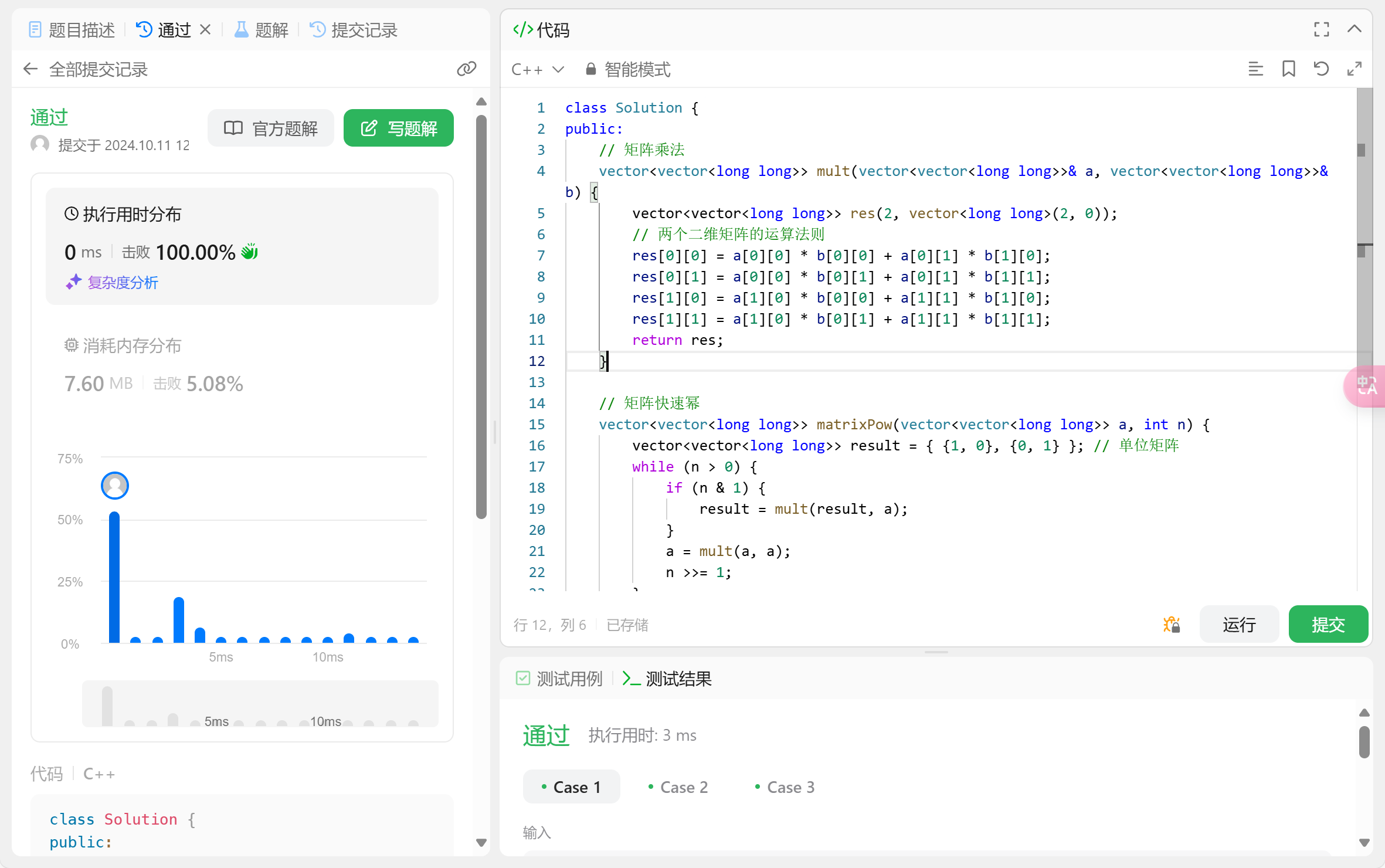 Note: Because its time complexity is
 O(logn), and O(n) already achieves 0ms, its superiority is not demonstrated in the test.
Because constructing the matrix incurs overhead, its superior time complexity only becomes apparent with large data. Therefore, with small data volumes, it may actually be slower than other implementation methods (for small data volumes, the dynamic programming implementation is better).
Other Implementations
In addition to the ordinary formula for the Fibonacci sequence, there is another formula:
 (Excerpted from the article: https://zhuanlan.zhihu.com/p/26679684)
Using this implementation method can reduce the time complexity to O(1). I will not demonstrate the code here; you can check it yourself if needed.
Summary
The above is my explanation of the algorithm implementation for the Fibonacci sequence. I hope it gives you a deeper understanding of the Fibonacci sequence.
